Reading Ice by Its Light
We think of snow and ice as simple materials, and they can look that way to the naked eye — but pointing a spectrometer at them reveals complex structure. Absorption bands appear at precise infrared wavelengths. Impurities carve signatures into the visible waveband. The shape of the reflected spectrum is a coded message about what the surface is made of, how old it is, and what is living on it. Radiative transfer is the physics that decodes it.
That decoding matters across a surprisingly wide range of science and engineering — far beyond the traditional framing of climate feedback loops.
Monitoring a changing Arctic
Satellite-derived spectral albedo is one of the most direct indicators of ice sheet and sea ice health. By tracking how reflectance changes year on year, researchers can map where melt is accelerating, separate the contributions of grain metamorphism, dust deposition, and biological darkening, and feed physically consistent albedo into ice-sheet models.
Exploring ice surface ecosystems
Glacier algae, snow algae, cyanobacteria, and even ice-worm communities are reshaping our understanding of life at the margins. These organisms darken the ice and their unique pigment spectra offer a way to map their distribution from space. Radiative transfer models are the bridge between a pigment absorption spectrum measured in a lab and a satellite image covering 100 m² of the Greenland ice sheet.
Predicting downstream flows and new landscapes
How much meltwater a glacier produces each summer depends directly on how much solar energy it absorbs — which depends on albedo. Accurate spectral albedo feeds into energy-balance melt models that predict river discharge, hydropower availability, irrigation supply, and flood risk for downstream communities. As glaciers retreat and new land is exposed, the same physics governs how quickly deglaciated terrain transitions from high-albedo ice to low-albedo rock and pioneer vegetation — reshaping local hydrology and ecology in the process.
In each case the starting point is the same: a physical model that connects the microphysical state of ice to the spectral signal a sensor records. BioSNICAR is that model — open-source, Python-native, and designed to span the full pipeline from ice crystal properties to satellite-band retrievals.
Every spectrum on this page was generated by BioSNICAR's adding-doubling radiative transfer solver — the same code used in peer-reviewed cryosphere research. All spectra are physically accurate, not toy approximations.
The Spectral Fingerprint of Ice
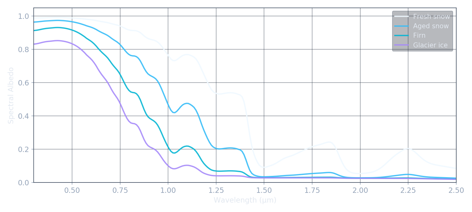
Ice doesn't just reflect light uniformly — it absorbs at very specific wavelengths determined by the molecular vibrations of the H₂O crystal lattice. The imaginary part of ice's complex refractive index creates absorption bands at 1.03, 1.25, 1.5, and 2.0 µm. Between these bands, albedo partially recovers. This characteristic structure is the spectral fingerprint of ice.
The depth of each absorption feature depends on the optical path length through ice before a photon is scattered back out. Larger grains mean longer transport paths in the ice, and lower albedo in the near-infrared. The visible region (below 0.7 µm) is nearly unaffected because ice is almost perfectly transparent at those wavelengths — photons scatter off grain surfaces and escape the ice without being absorbed.
This wavelength dependence is what makes spectral remote sensing so powerful for snow and ice. A single broadband albedo measurement can't tell you why the surface is dark — grain growth, impurities, and thin snow over rock all lower the average. But the spectral shape is unique to each process: grain growth deepens NIR features while leaving the visible untouched; black carbon suppresses the visible while barely touching the NIR. The spectrum is the diagnostic.
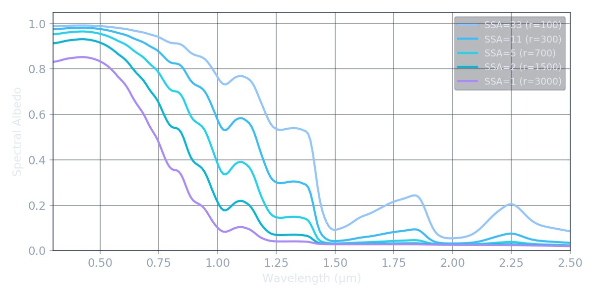
Try it: drag the grain-size slider
Each curve is a real BioSNICAR simulation. Watch how the near-infrared absorption features deepen as grains grow.
SSA = 3 / (r × ρice), in m² kg⁻¹, combines grain size and ice density into the single parameter that best predicts spectral shape. Fresh snow: SSA ≈ 30–60 (tiny grains, lots of scattering). Glacier ice: SSA ≈ 0.5–3 (large grains, deep absorption). SSA is what satellite retrievals actually constrain — not grain radius or density individually, because different (r, ρ) pairs yielding the same SSA produce identical spectra.
Impurities: When Snow Gets Dirty
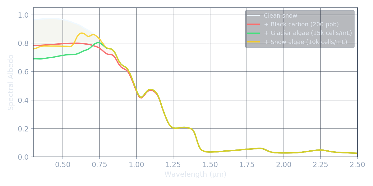
Pure ice absorbs almost nothing in the visible — that's why snow is white. But even trace amounts of light-absorbing particles (LAPs) can dramatically darken the surface. A dusting of black carbon at just 10 parts per billion measurably reduces albedo; a heavy algae bloom can halve it.
Crucially, each impurity type has a distinct spectral signature. Black carbon absorbs with a smooth power-law across all visible wavelengths. Algal pigments create characteristic absorption features at specific wavelengths corresponding to carotenoids (~470 nm) and chlorophyll-a (~670 nm). These spectral differences are what make it possible — in principle — to identify and quantify impurities from satellite data.
Black Carbon
From fossil fuel combustion, wildfires, and agricultural burning. Absorbs across the full visible spectrum with a λ−1 wavelength dependence. Even 10 ppb measurably darkens snow; concentrations above 100 ppb cause visible greying.
Snow Algae
Unicellular green algae (Chlamydomonas nivalis and relatives) that accumulate red astaxanthin pigment as a sunscreen. Causes "watermelon snow" — pink-red patches on seasonal snowpacks. Absorbs broadly around 480 nm and 680 nm.
Glacier Algae
Elongated filamentous cells (Ancylonema nordenskiöldii) that bloom on bare melting ice. Packed with purpurogallin-type phenolic pigments absorbing 350–700 nm, creating a brown-purple colour. A major driver of Greenland ice sheet darkening.
Mineral Dust
Wind-deposited particles from deserts, exposed moraines, and volcanic ash. Absorbs with a broad, featureless spectrum that overlaps heavily with grain-size effects — making dust the hardest impurity to retrieve from spectral data alone.
Try it: add black carbon
Drag the slider to see how increasing black carbon concentration darkens the visible spectrum while leaving the NIR largely unchanged. All curves are real BioSNICAR output.
Try it: grow an algae bloom
Watch how glacier algae progressively darken the visible spectrum, with absorption concentrated around the pigment wavelengths (470 nm and 670 nm).
What Satellites See
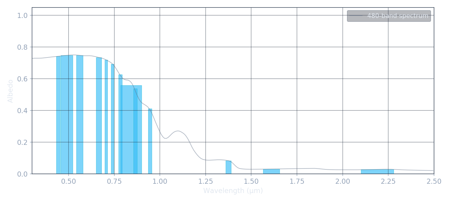
Satellites don't measure continuous spectra. They collect light in discrete spectral bands, each integrating the spectrum over a wavelength range weighted by the sensor's spectral response function and the incoming solar flux. Sentinel-2, for example, compresses 480 spectral values into just 13 numbers.
This compression is lossy — fine spectral features disappear — but the band values still encode enough information to retrieve 2–3 physical parameters. The key is choosing the right bands: SWIR bands (1.6, 2.2 µm) are essential for constraining SSA, while visible bands capture impurity darkening.
Different platforms offer different trade-offs. BioSNICAR's
to_platform() function handles the spectral convolution
for all of them:
Sentinel-2 MSI
13 bands, 10–60 m resolution, 5-day revisit. The current workhorse for snow/ice retrieval thanks to SWIR coverage and high spatial resolution.
Landsat 8 OLI
7 bands, 30 m resolution, 16-day revisit. Decades of continuous archive make it invaluable for long-term albedo trend analysis.
MODIS
7 land bands + 3 broadband, 500 m resolution, daily global coverage. The go-to sensor for large-scale, high-cadence albedo mapping.
Climate Models
CESM (2 or 14 bands), MAR (4 bands), HadCM3 (6 bands). BioSNICAR provides albedo at the spectral resolution each model's radiation scheme requires.
The Inverse Problem
The forward problem is straightforward: given ice properties, BioSNICAR computes the spectrum in ~0.5 seconds. The inverse problem asks the harder question: given a satellite observation, what are the ice properties that produced it?
geometry
BioSNICAR
spectrum
to_platform()bands
Inversion reverses this pipeline: an optimiser adjusts the physical parameters until the forward model's predicted bands match the satellite observation. But the challenges are real:
Parameter degeneracy
Different parameter combinations can produce identical spectra. Grain radius and density trade off against each other along constant-SSA contours. The solution: retrieve SSA directly rather than the individual components.
Information limits
PCA analysis shows that 13 Sentinel-2 bands carry only ~3–4 independent degrees of freedom. You cannot retrieve more parameters than the data can constrain — fix everything else with ancillary data.
BioSNICAR solves the speed problem with a machine-learning emulator (PCA + neural network) trained on forward-model samples. The emulator reproduces the full solver at 50,000× the speed (~10 µs per evaluation), making optimisation, MCMC uncertainty quantification, and large-scale retrieval campaigns practical.
Retrieve SSA, not grain radius (Section 11 of the
remote sensing notebook explains why). Fix solar zenith from
ephemeris data. Mask atmospheric absorption bands at 1.4 and
1.9 µm. Use fixed_params to constrain what you
know. Start with 1–2 free parameters and add more only if the
data supports it.
Try it: be the retrieval algorithm
The yellow curve is a mystery observation from a real BioSNICAR simulation. Adjust the two sliders to find the grain size and black carbon concentration that best match it. The blue curve is your current guess; the cost value tells you how close you are. Can you get the cost below 0.01?
BioSNICAR: The Complete Toolkit
BioSNICAR is an open-source Python implementation of the SNICAR radiative transfer model, extended with biological impurities (snow algae, glacier algae), a machine-learning emulator, satellite band convolution for 8 platforms, and a full inverse-modelling framework. It runs the complete pipeline from ice crystal properties to satellite-band retrievals in a single package.
Forward Model
Adding-doubling solver with delta-Eddington scaling. Handles multi-layer snowpacks with Fresnel boundaries, 4 impurity types (BC, dust, snow algae, glacier algae), liquid water coatings, and 480 spectral bands from 0.2–5.0 µm.
Band Convolution
8 platforms: Sentinel-2, Sentinel-3, Landsat 8, MODIS, CESM (2-band and RRTMG 14-band), MAR, and HadCM3. SRF convolution for satellites, flux-weighted interval averaging for GCMs. Spectral indices (NDSI, NDVI, Impurity Index) computed automatically.
ML Emulator
PCA compression + multi-layer perceptron trained on Latin
hypercube samples from the forward model. 50,000× faster than
the full solver. Build custom emulators for any parameter
subset via Emulator.build().
Inverse Framework
retrieve() dispatches to spectral or band-mode
cost functions with log-space optimisation, Hessian or MCMC
uncertainty, wavelength masking, and fixed parameters.
Hybrid DE + L-BFGS-B for global-to-local convergence.
Quick Start
# Clone and install
git clone https://github.com/jmcook1186/biosnicar-py.git
cd biosnicar-py
pip install -e .

# Forward model → spectral albedo
from biosnicar import run_model

outputs = run_model(rds=500, rho=600, black_carbon=50, solzen=50)

# Convert to Sentinel-2 bands
s2 = outputs.to_platform("sentinel2")
print(f"NDSI = {s2.NDSI:.3f}")

# Retrieve SSA from observations
from biosnicar.inverse import retrieve
result = retrieve(observed, ["ssa", "black_carbon"], emulator,
                  platform="sentinel2")